Objective
The main goal of this post is to:
- Show one way of performing variable selection in a competing risks regression model
- Evaluate the predictive performance for a list of models using resampling methods
What the data looks like
We will use the bmtcrr dataset from the casebase package available on CRAN. Here is what the data looks like:
pacman::p_load(casebase)
head(bmtcrr)
## Sex D Phase Age Status Source ftime
## 1 M ALL Relapse 48 2 BM+PB 0.67
## 2 F AML CR2 23 1 BM+PB 9.50
## 3 M ALL CR3 7 0 BM+PB 131.77
## 4 F ALL CR2 26 2 BM+PB 24.03
## 5 F ALL CR2 36 2 BM+PB 1.47
## 6 M ALL Relapse 17 2 BM+PB 2.23We will perform a competing risk analysis on data from 177 patients who received a stem cell transplant for acute leukemia. The event of interest in relapse, but other competing causes (e.g. transplant-related death) need to be taken into account. We also want to take into account the effect of several covariates such as Sex, Disease (lymphoblastic or myeloblastic leukemia, abbreviated as ALL and AML, respectively), Phase at transplant (Relapse, CR1, CR2, CR3), Source of stem cells (bone marrow and peripheral blood, coded as BM+PB, or peripheral blood, coded as PB), and Age. Below, is the Table 1:
| Variable | Description | Statistical summary |
|---|---|---|
| Sex | Sex |
M=Male (100) F=Female (77) |
| D | Disease |
ALL (73) AML (104) |
| Phase | Phase |
CR1 (47) CR2 (45) CR3 (12) Relapse (73) |
| Source | Type of transplant |
BM+PB (21) PB (156) |
| Age | Age of patient (years) |
4–62 30.47 (13.04) |
| Ftime | Failure time (months) |
0.13–131.77 20.28 (30.78) |
| Status | Status indicator |
0=censored (46) 1=relapse (56) 2=competing event (75) |
The statistical summary is generated differently for continuous and categorical variables:
-
For continuous variables, we are given the range, followed by the mean and standard deviation.
-
For categorical variables, we are given the counts for each category.
Variable Selection
Here we compare the variables selected using three methods:
- Full model: contains all of the predictors and no variable selection is being done.
- Backward selection based on the AIC.
- Backward selection based on the BIC.
Load the necessary packages
pacman::p_load(riskRegression) # for Fine-Gray Regression (FGR)
pacman::p_load(prodlim) # for Hist function
pacman::p_load(lava) # not sure, but its needed
pacman::p_load(cmprsk) # competing risks
pacman::p_load(crrstep) # for variable selection in FGR
pacman::p_load(pec) # for resampling metrics
Prepare the data
This step is required if you have categorical data. You must convert the factors into indicator variables using model.matrix:
fmla <- as.formula( ~ ftime + Status + Sex +
                      Phase + Source + Age + D)

# remove intercept
bmtcrr.expanded <- as.data.frame(model.matrix(fmla,
                              data = bmtcrr)[,-1])
head(bmtcrr.expanded)
## ftime Status SexM PhaseCR2 PhaseCR3 PhaseRelapse SourcePB Age DAML
## 1 0.67 2 1 0 0 1 0 48 0
## 2 9.50 1 0 1 0 0 0 23 1
## 3 131.77 0 1 0 1 0 0 7 0
## 4 24.03 2 0 1 0 0 0 26 0
## 5 1.47 2 0 1 0 0 0 36 0
## 6 2.23 2 1 0 0 1 0 17 0# get the names of the covariates only
covariates <- setdiff(colnames(bmtcrr.expanded),
c("ftime","Status"))Run the variable selection
# formula for the Full model
(ff <- as.formula(paste0("Hist(ftime, Status) ~ ",
                 paste(covariates, collapse = "+"))))
## Hist(ftime, Status) ~ SexM + PhaseCR2 + PhaseCR3 + PhaseRelapse +
## SourcePB + Age + DAML# Fit full model with Fine-Grey regression model
fg <- riskRegression::FGR(ff, cause = 1, data = bmtcrr.expanded)
# Backward selection based on the AIC
sfgAIC <- pec::selectFGR(ff, cause = 1, data = bmtcrr.expanded,
rule = "AIC", direction = "backward")
# Final FGR-model with selected variables
sfgAIC$fit ##
## Right-censored response of a competing.risks model
##
## No.Observations: 177
##
## Pattern:
##
## Cause event right.censored
## 1 56 0
## 2 75 0
## unknown 0 46
##
##
## Fine-Gray model: analysis of cause 1
##
## Competing Risks Regression
##
## Call:
## riskRegression::FGR(formula = Hist(ftime, Status) ~ PhaseRelapse +
## SourcePB + Age + DAML, data = data, cause = cause)
##
## coef exp(coef) se(coef) z p-value
## PhaseRelapse 1.021 2.776 0.2724 3.75 0.00018
## SourcePB 0.889 2.434 0.5400 1.65 0.10000
## Age -0.019 0.981 0.0117 -1.63 0.10000
## DAML -0.463 0.630 0.2979 -1.55 0.12000
##
## exp(coef) exp(-coef) 2.5% 97.5%
## PhaseRelapse 2.776 0.360 1.628 4.73
## SourcePB 2.434 0.411 0.845 7.01
## Age 0.981 1.019 0.959 1.00
## DAML 0.630 1.588 0.351 1.13
##
## Num. cases = 177
## Pseudo Log-likelihood = -267
## Pseudo likelihood ratio test = 24.1 on 4 df,
##
## Convergence: TRUE# Backward selection based on the BIC
sfgBIC <- pec::selectFGR(ff, cause = 1, data = bmtcrr.expanded,
rule = "BIC", direction = "backward")
# Final FGR-model with selected variables
sfgBIC$fit##
## Right-censored response of a competing.risks model
##
## No.Observations: 177
##
## Pattern:
##
## Cause event right.censored
## 1 56 0
## 2 75 0
## unknown 0 46
##
##
## Fine-Gray model: analysis of cause 1
##
## Competing Risks Regression
##
## Call:
## riskRegression::FGR(formula = Hist(ftime, Status) ~ PhaseRelapse +
## SourcePB + Age + DAML, data = data, cause = cause)
##
## coef exp(coef) se(coef) z p-value
## PhaseRelapse 1.021 2.776 0.2724 3.75 0.00018
## SourcePB 0.889 2.434 0.5400 1.65 0.10000
## Age -0.019 0.981 0.0117 -1.63 0.10000
## DAML -0.463 0.630 0.2979 -1.55 0.12000
##
## exp(coef) exp(-coef) 2.5% 97.5%
## PhaseRelapse 2.776 0.360 1.628 4.73
## SourcePB 2.434 0.411 0.845 7.01
## Age 0.981 1.019 0.959 1.00
## DAML 0.630 1.588 0.351 1.13
##
## Num. cases = 177
## Pseudo Log-likelihood = -267
## Pseudo likelihood ratio test = 24.1 on 4 df,
##
## Convergence: TRUE# create list of models
models_list <- list(full.model = fg, selectedAIC = sfgAIC, selectedBIC = sfgBIC)Bootstrap cross-validation performance
## Lower Brier Score is better
## The reference model is without any covariates
set.seed(7)
p2 <- pec::pec(models_list,
               formula = ff,
               data = bmtcrr.expanded,
               B = 5,
splitMethod = "Boot632")p2##
## Prediction error curves
##
## Prediction models:
##
## Reference full.model selectedAIC selectedBIC
## Reference full.model selectedAIC selectedBIC
##
## Right-censored response of a competing.risks model
##
## No.Observations: 177
##
## Pattern:
##
## Cause event right.censored
## 1 56 0
## 2 75 0
## unknown 0 46
##
## IPCW: cox model
##
## Method for estimating the prediction error:
##
## Bootstrap cross-validation
##
## Type: resampling
## Bootstrap sample size: 177
## No. bootstrap samples: 5
## Sample size: 177
##
## Cumulative prediction error, aka Integrated Brier score (IBS)
## aka Cumulative rank probability score
##
## Range of integration: 0 and time=121.1 :
##
##
## Integrated Brier score (crps):
##
## IBS[0;time=121.1)
## Reference 0.200
## full.model 0.190
## selectedAIC 0.195
## selectedBIC 0.195plot(p2)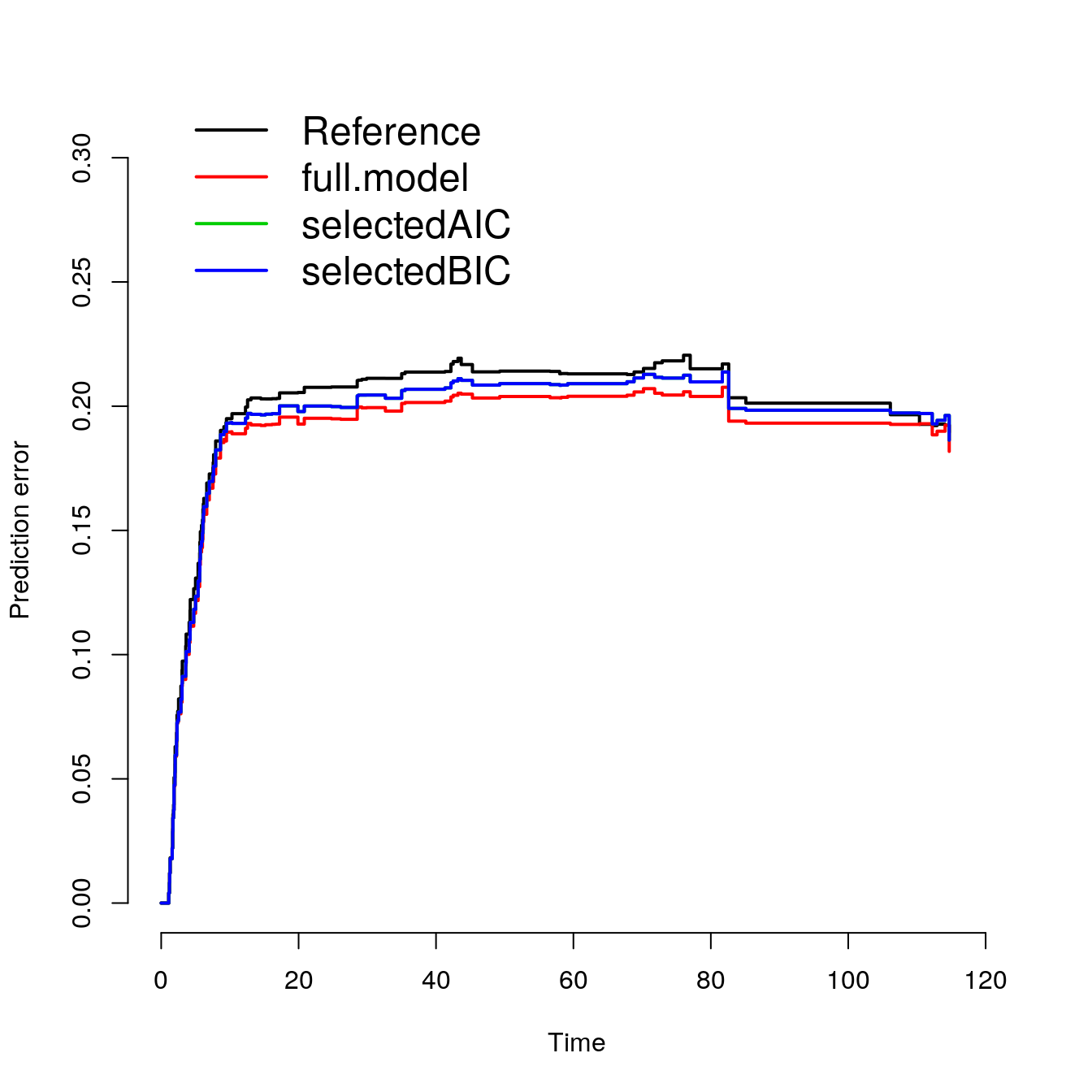
Calibration Plot
calPlot(models_list,
        formula=ff, splitMethod = "BootCv", B=5)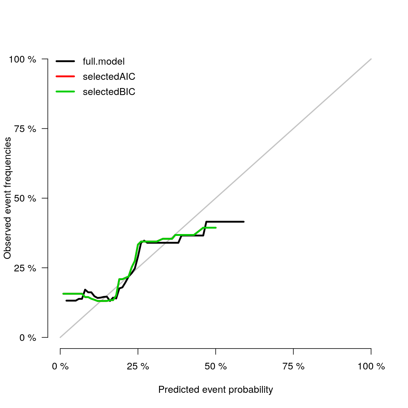
Observed vs. Predicted for each Method
# Full Model
b1 <- pec::calPlot(models_list[[1]],
              formula = ff,
              bars = TRUE,
              hanging = FALSE)
print(b1)
##
## Calibration of risk predictions for 177 subjects.
##
## Until time 6.63 a total of 88 were observed event-free,
## - a total of 37 were observed to have the event of interest (cause: 1),
## - a total of 52 had a competing risk
## - a total of 0 were lost to follow-up.
##
## Average predictions and outcome in prediction quantiles:
##
## $Model.1
## Pred Obs
## [0.0456,0.087] 0.07135827 0.05555556
## (0.087,0.103] 0.09430400 0.11111111
## (0.103,0.124] 0.11175112 0.11764706
## (0.124,0.146] 0.13458330 0.22222222
## (0.146,0.18] 0.16277313 0.00000000
## (0.18,0.209] 0.19717791 0.11764706
## (0.209,0.24] 0.22618829 0.27777778
## (0.24,0.292] 0.26695026 0.41176471
## (0.292,0.45] 0.35246826 0.27777778
## (0.45,0.593] 0.50029249 0.50000000
##
##
## Outcome frequencies (Obs) were obtained with the Aalen-Johansen method.plot(b1)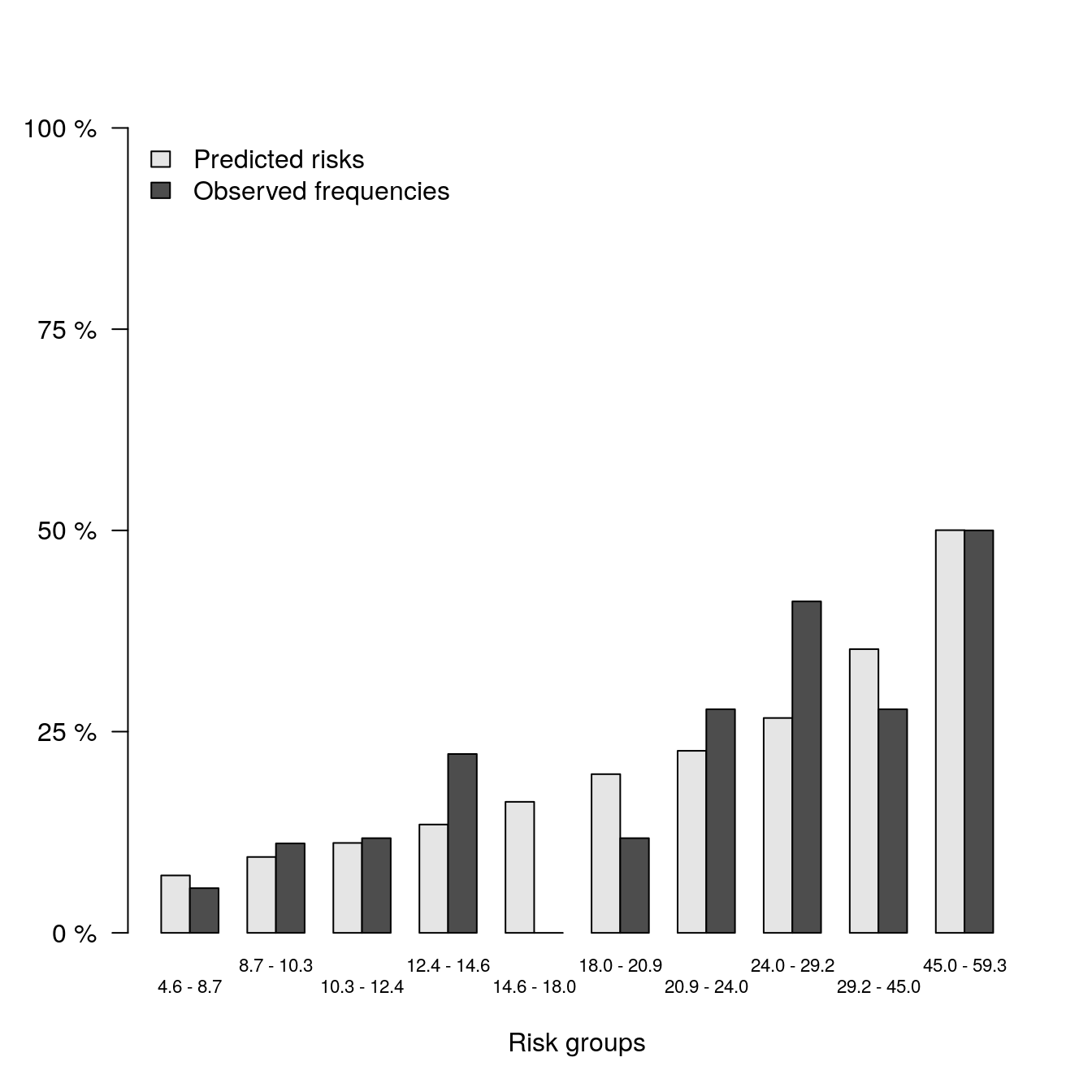
# Selected AIC Model
b2 <- pec::calPlot(models_list[[2]],
                   formula = ff,
                   bars = TRUE,
                   hanging = FALSE)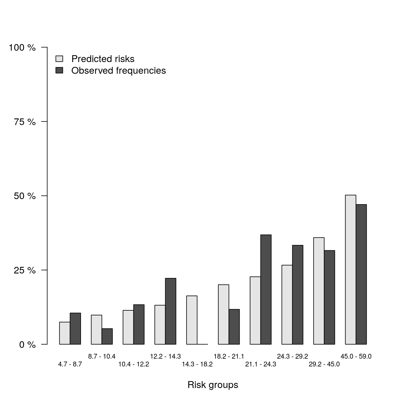
print(b2)##
## Calibration of risk predictions for 177 subjects.
##
## Until time 6.63 a total of 88 were observed event-free,
## - a total of 37 were observed to have the event of interest (cause: 1),
## - a total of 52 had a competing risk
## - a total of 0 were lost to follow-up.
##
## Average predictions and outcome in prediction quantiles:
##
## $Model.1
## Pred Obs
## [0.0467,0.087] 0.07468652 0.10526316
## (0.087,0.104] 0.09825360 0.05263158
## (0.104,0.122] 0.11424004 0.13333333
## (0.122,0.143] 0.13148919 0.22222222
## (0.143,0.182] 0.16298969 0.00000000
## (0.182,0.211] 0.20063789 0.11764706
## (0.211,0.243] 0.22723987 0.36842105
## (0.243,0.292] 0.26637445 0.33333333
## (0.292,0.45] 0.35913229 0.31578947
## (0.45,0.59] 0.50223610 0.47058824
##
##
## Outcome frequencies (Obs) were obtained with the Aalen-Johansen method.plot(b2)
# Selected BIC Model
b3 <- pec::calPlot(models_list[[3]],
formula = ff,
bars = TRUE,
hanging = FALSE)
print(b3)##
## Calibration of risk predictions for 177 subjects.
##
## Until time 6.63 a total of 88 were observed event-free,
## - a total of 37 were observed to have the event of interest (cause: 1),
## - a total of 52 had a competing risk
## - a total of 0 were lost to follow-up.
##
## Average predictions and outcome in prediction quantiles:
##
## $Model.1
## Pred Obs
## [0.0467,0.087] 0.07468652 0.10526316
## (0.087,0.104] 0.09825360 0.05263158
## (0.104,0.122] 0.11424004 0.13333333
## (0.122,0.143] 0.13148919 0.22222222
## (0.143,0.182] 0.16298969 0.00000000
## (0.182,0.211] 0.20063789 0.11764706
## (0.211,0.243] 0.22723987 0.36842105
## (0.243,0.292] 0.26637445 0.33333333
## (0.292,0.45] 0.35913229 0.31578947
## (0.45,0.59] 0.50223610 0.47058824
##
##
## Outcome frequencies (Obs) were obtained with the Aalen-Johansen method.plot(b3)