This post shows how to calculate the Net Re-Classification Index and Goodness-of-Fit Test (Hosmer-Lemeshow Test) for logistic regression models. In addition, we show how to plot the calibration curves.
#  load packages ----------------------------------------------------------

if (!requireNamespace("pacman", quietly = TRUE)) {
  install.packages("pacman")
}
pacman::p_load(PredictABEL)
pacman::p_load(aod)
pacman::p_load(ggplot2)

# packages for ggplot2 themes
pacman::p_load(ggrepel)

# colors and themes -------------------------------------------------------

# color blind palette
cbbPalette <- c("#999999", "#E69F00", "#56B4E9", "#009E73", "#F0E442", "#0072B2", "#D55E00", "#CC79A7")

# my theme defaults
gg_sy <- theme(legend.position = "bottom",
               axis.text = element_text(size = 20),
               axis.title = element_text(size = 20),
               legend.text = element_text(size = 20),
               legend.title = element_text(size = 20))


#  load data --------------------------------------------------------------


mydata <- read.csv("https://stats.idre.ucla.edu/stat/data/binary.csv")
## view the first few rows of the data
head(mydata)
## admit gre gpa rank
## 1 0 380 3.61 3
## 2 1 660 3.67 3
## 3 1 800 4.00 1
## 4 1 640 3.19 4
## 5 0 520 2.93 4
## 6 1 760 3.00 2mydata$rank <- factor(mydata$rank)
mydata$admitf <- factor(mydata$admit, levels = c(0,1), labels = c("no admit", "admit"))
# without rank
m1 <- glm(admit ~ gre + gpa, data = mydata, family = "binomial")
preds_m1 <- predict(m1, type = "response") # predicted probs from model 1
# with rank
m2 <- glm(admit ~ gre + gpa + rank, data = mydata, family = "binomial")
preds_m2 <- predict(m2, type = "response") # predicted probs from model 2
# Calibration plots and Hosmer Lemeshow test ------------------------------
# In this example, we see that the $Chi_square value is smaller for m2, compared to m1
# The null hypothesis is that we have a good fit. So the larger the p-value, the smaller the
# Chi_square statistic, the better the fit. So we can say that rank has added value to the model
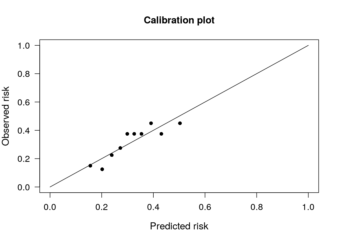
# Calibration plot for m1
PredictABEL::plotCalibration(data = as.matrix(mydata$admit), # observed response
cOutcome = 1, # the category corresponding to outcome of interest
predRisk = preds_m1, # predicted probs
groups = 10 # number of groups to bin the predicted probabilities into, usually 10 is default
)## $Table_HLtest
## total meanpred meanobs predicted observed
## [0.0978,0.184) 40 0.156 0.150 6.25 6
## [0.1839,0.224) 40 0.202 0.125 8.09 5
## [0.2241,0.254) 40 0.239 0.225 9.56 9
## [0.2536,0.289) 40 0.272 0.275 10.89 11
## [0.2894,0.311) 40 0.299 0.375 11.97 15
## [0.3110,0.341) 40 0.326 0.375 13.04 15
## [0.3406,0.370) 40 0.354 0.375 14.16 15
## [0.3702,0.408) 40 0.391 0.450 15.64 18
## [0.4079,0.461) 40 0.431 0.375 17.26 15
## [0.4614,0.555] 40 0.503 0.450 20.13 18
##
## $Chi_square
## [1] 4.706
##
## $df
## [1] 8
##
## $p_value
## [1] 0.7885# Calibration plot for m2
PredictABEL::plotCalibration(data = as.matrix(mydata$admit), # observed response
cOutcome = 1, # the category corresponding to outcome of interest
predRisk = preds_m1, # predicted probs
groups = 10 # number of groups to bin the predicted probabilities into, usually 10 is default, so you will see 10 categories and 10 points on the calibration plot
)
## $Table_HLtest
##                total meanpred meanobs predicted observed
## [0.0978,0.184)    40    0.156   0.150      6.25        6
## [0.1839,0.224)    40    0.202   0.125      8.09        5
## [0.2241,0.254)    40    0.239   0.225      9.56        9
## [0.2536,0.289)    40    0.272   0.275     10.89       11
## [0.2894,0.311)    40    0.299   0.375     11.97       15
## [0.3110,0.341)    40    0.326   0.375     13.04       15
## [0.3406,0.370)    40    0.354   0.375     14.16       15
## [0.3702,0.408)    40    0.391   0.450     15.64       18
## [0.4079,0.461)    40    0.431   0.375     17.26       15
## [0.4614,0.555]    40    0.503   0.450     20.13       18
##
## $Chi_square
## [1] 4.706
##
## $df
## [1] 8
##
## $p_value
## [1] 0.7885
# Boxplots for discrimination ---------------------------------------------
df1 <- data.frame(admit = mydata$admitf,
model = "w/o rank",
predicted = preds_m1,
stringsAsFactors = FALSE)
df2 <- data.frame(admit = mydata$admitf,
model = "with rank",
predicted = preds_m2,
stringsAsFactors = FALSE)
dfplot <- rbind(df1, df2)
dfplot$model <- factor(dfplot$model)
ggplot(dfplot, aes(x = admit, y = predicted, fill = model)) +
geom_boxplot() +
scale_fill_manual(values=cbbPalette[c(3,7)], guide=guide_legend(ncol = 2)) +
labs(x="", y="Predicted probability",
title="Predicted probability by observed outcome for each model",
subtitle="Based on logistic regression model adjusted for GRE and GPA",
caption="") +
# theme_ipsum_rc() +
theme(legend.position = "bottom",
axis.text = element_text(size = 20),
axis.title = element_text(size = 20),
legend.text = element_text(size = 20),
legend.title = element_text(size = 20))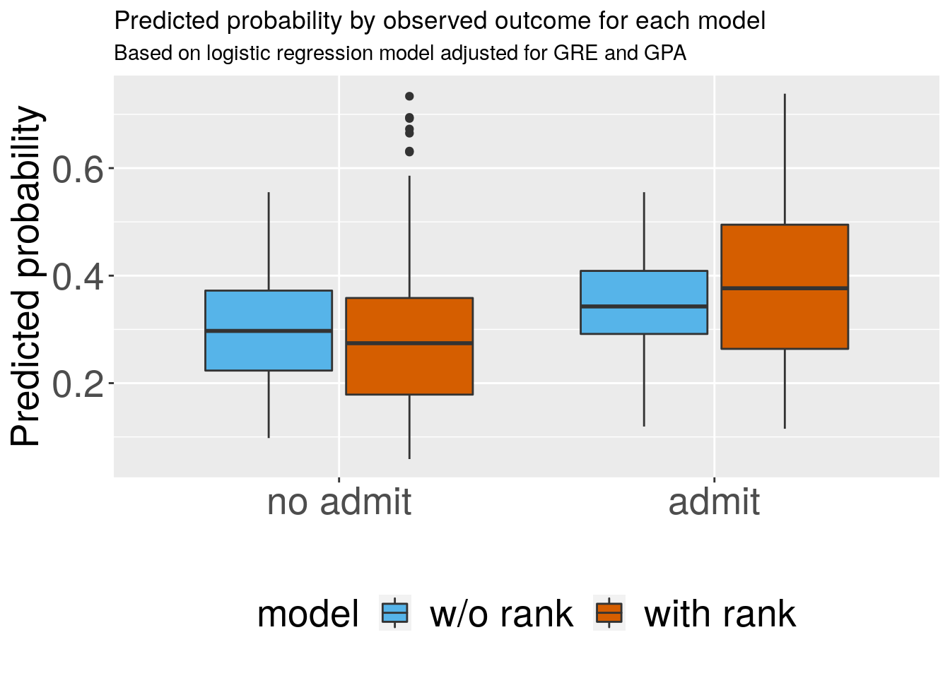
# Net reclassification index ----------------------------------------------

#' Re-classfication tables quantify the model improvement of one model over
#' another by counting the number of individuals who move to another risk
#' category or remain in the same risk category as a result of updating the risk
#' model. Any _upward_ movement in categories for event subjects (i.e. those
#' with admit=1) implies improved classification, and any _downward_ movement
#' indicates worse reclassification. The interpretation is opposite for people
#' who do not develop events (admit = 0). Smaller p-values indicate better
#' reclassification accuracy.
#'

PredictABEL::reclassification(data = as.matrix(mydata$admit),
                              cOutcome = 1,
                              predrisk1 = preds_m1, # original model
                              predrisk2 = preds_m2, # updated model
                              cutoff = seq(0, 1, by = 0.20))
## _________________________________________
##
## Reclassification table
## _________________________________________
##
## Outcome: absent
##
## Updated Model
## Initial Model [0,0.2) [0.2,0.4) [0.4,0.6) [0.6,0.8) [0.8,1] % reclassified
## [0,0.2) 31 16 0 0 0 34
## [0.2,0.4) 52 99 24 0 0 43
## [0.4,0.6) 0 26 18 7 0 65
## [0.6,0.8) 0 0 0 0 0 NaN
## [0.8,1] 0 0 0 0 0 NaN
##
##
## Outcome: present
##
## Updated Model
## Initial Model [0,0.2) [0.2,0.4) [0.4,0.6) [0.6,0.8) [0.8,1] % reclassified
## [0,0.2) 7 2 0 0 0 22
## [0.2,0.4) 11 40 28 0 0 49
## [0.4,0.6) 0 11 15 13 0 62
## [0.6,0.8) 0 0 0 0 0 NaN
## [0.8,1] 0 0 0 0 0 NaN
##
##
## Combined Data
##
## Updated Model
## Initial Model [0,0.2) [0.2,0.4) [0.4,0.6) [0.6,0.8) [0.8,1] % reclassified
## [0,0.2) 38 18 0 0 0 32
## [0.2,0.4) 63 139 52 0 0 45
## [0.4,0.6) 0 37 33 20 0 63
## [0.6,0.8) 0 0 0 0 0 NaN
## [0.8,1] 0 0 0 0 0 NaN
## _________________________________________
##
## NRI(Categorical) [95% CI]: 0.2789 [ 0.1343 - 0.4235 ] ; p-value: 0.00016
## NRI(Continuous) [95% CI]: 0.4543 [ 0.2541 - 0.6545 ] ; p-value: 1e-05
## IDI [95% CI]: 0.0546 [ 0.0309 - 0.0783 ] ; p-value: 1e-05Further Reading (UPDATED January 10, 2020)
Good to raise aware of calibration but Hosmer-Lemeshow test doesn't assess calibration (and has many problems, e.g., summarised in Box G of https://t.co/4yiJe4bDu3), plus there a number of problems with the NRI (e.g., https://t.co/TkukdbV56l, https://t.co/EYyfx55BQT)
— Gary Collins 🇪🇺 (@GSCollins) September 6, 2019