Simulation function – response is a quadratic function of continuous predictor
sim_quadratic_logistic_data = function(sample_size = 25) {
  x = rnorm(n = sample_size)
  eta = -1.5 + 0.5 * x + x ^ 2 + rnorm(sample_size, sd = 2) # add some noise
  p = 1 / (1 + exp(-eta))
  y = rbinom(n = sample_size, size = 1, prob = p)
  data.frame(y.factor = factor(y, levels = 1:0, labels = c("COPD","control")), x = x, y = y)
}
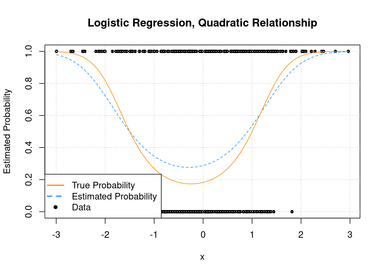
Fit once to see what the resulting predicted curve looks like
set.seed(42)
example_data <- sim_quadratic_logistic_data(sample_size = 500)
table(example_data$y.factor)
##
##    COPD control
##     209     291
fit_glm <- glm(y ~ x + I(x^2), data = example_data, family = binomial)
summary(fit_glm)
##
## Call:
## glm(formula = y ~ x + I(x^2), family = binomial, data = example_data)
##
## Deviance Residuals:
##     Min       1Q   Median       3Q      Max
## -2.0555  -0.8862  -0.8084   1.2208   1.6041
##
## Coefficients:
##             Estimate Std. Error z value Pr(>|z|)
## (Intercept)  -0.9058     0.1255  -7.217 5.30e-13 ***
## x             0.3904     0.1118   3.491 0.000482 ***
## I(x^2)        0.6619     0.1009   6.558 5.45e-11 ***
## ---
## Signif. codes:  0 '***' 0.001 '**' 0.01 '*' 0.05 '.' 0.1 ' ' 1
##
## (Dispersion parameter for binomial family taken to be 1)
##
##     Null deviance: 679.64  on 499  degrees of freedom
## Residual deviance: 609.91  on 497  degrees of freedom
## AIC: 615.91
##
## Number of Fisher Scoring iterations: 4
plot(y ~ x, data = example_data,
     pch = 20, ylab = "Estimated Probability",
     main = "Logistic Regression, Quadratic Relationship")
grid()
curve(predict(fit_glm, data.frame(x), type = "response"),
      add = TRUE, col = "dodgerblue", lty = 2)
curve(boot::inv.logit(-1.5 + 0.5 * x + x ^ 2),
      add = TRUE, col = "darkorange", lty = 1)
legend("bottomleft", c("True Probability", "Estimated Probability", "Data"), lty = c(1, 2, 0),
       pch = c(NA, NA, 20), lwd = 2, col = c("darkorange", "dodgerblue", "black"))
Run cross-validation experiment once
if(!requireNamespace("pacman")) install.packages("pacman")
## Loading required namespace: pacman
pacman::p_load(caret)
pacman::p_load(MLmetrics)
pacman::p_load(dplyr)
pacman::p_load(tidyr)

# function that returns the metrics of interest
MySummary <- function (data, lev = NULL, model = NULL) {

  PPV = caret::posPredValue(data = data$pred,
                            reference = data$obs)
  NPV = caret::negPredValue(data = data$pred,
                            reference = data$obs)

  tt <- table(data$pred, data$obs)
  n_call_COPD <- sum(tt[1,]) # number of 'positives' called by the model
  n_call_control <- sum(tt[2,]) # number of 'negatives' called by the model

  c(PPV = PPV,
    NPV = NPV,
    Macro = (PPV + NPV) / 2, # JH calls this ave.suuccess12
    SE2_Macro =  (1/2^2) * (PPV * (1-PPV) / n_call_COPD + NPV * (1-NPV) / n_call_control) # JH calls this var.ave.success
  )
}
set.seed(42)

# sample size
N <- 500

# folds
K <- 5

# simulate data
df <- sim_quadratic_logistic_data(sample_size = N)

# fit the model with cross-validated metrics
fit <- caret::train(y.factor ~ x + I(x^2),
                    data = df,
                    method = "glm",
                    family = "binomial",
                    trControl = trainControl(method = "cv",
                                             number = K,
                                             savePredictions = TRUE,
                                             summaryFunction = MySummary,
                                             classProbs = TRUE))

fit$resample
##         PPV       NPV     Macro   SE2_Macro Resample
## 1 0.7307692 0.6891892 0.7099792 0.002615458    Fold1
## 2 0.5000000 0.6000000 0.5500000 0.003875000    Fold2
## 3 0.5652174 0.6282051 0.5967113 0.003419760    Fold3
## 4 0.8400000 0.7297297 0.7848649 0.002010298    Fold4
## 5 0.5909091 0.6282051 0.6095571 0.003495596    Fold5
Run CV experiment many times
set.seed(42)
n.samples <- 400 # number of replications
# sample size
N <- 500
# folds
K <- 5
# repeat experiment several times
res.list <- replicate(n.samples, expr = {
# simulate data with samp size
df <- sim_quadratic_logistic_data(sample_size = N)
# fit the model with cross-validated metrics
fit <- caret::train(y.factor ~ x + I(x^2),
data = df,
method = "glm",
family = "binomial",
trControl = trainControl(method = "cv",
number = K,
savePredictions = TRUE,
summaryFunction = MySummary,
classProbs = TRUE))
data.frame(
SE_pbar = sqrt((1/K)*mean(fit$resample$SE2_Macro)), # model based (what the reviewer suggested)
SEM = sd(fit$resample$Macro) / sqrt(K), # what we did aka the Standard error of the mean
corr_ppv_npv = cor(fit$resample$PPV, fit$resample$NPV)
)
}, simplify = FALSE)
res <- do.call(rbind, res.list) %>%
mutate(replicate = 1:n())
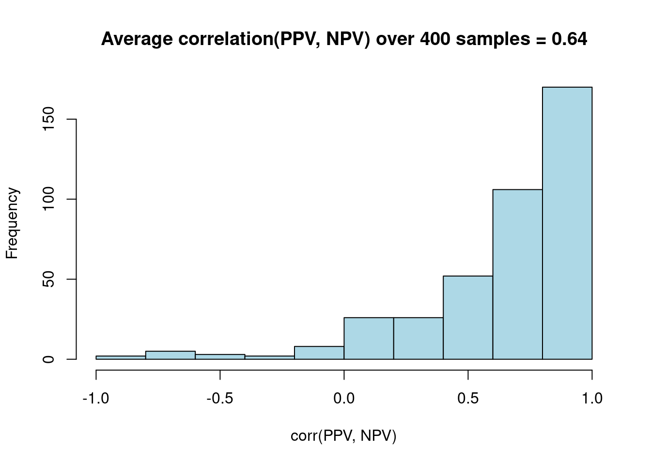
hist(res$corr_ppv_npv,
col = "lightblue",
xlab = "corr(PPV, NPV)",
main = sprintf("Average correlation(PPV, NPV) over %i samples = %0.2f",n.samples, mean(res$corr_ppv_npv)))
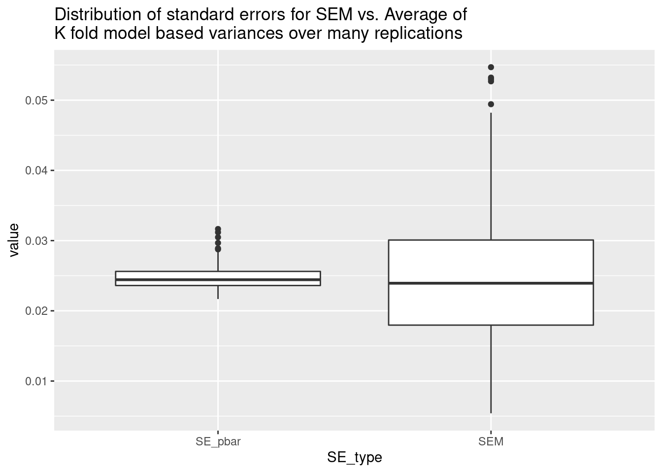
res %>%
  dplyr::select(replicate, SE_pbar, SEM) %>%
  tidyr::pivot_longer(cols = -1, names_to = "SE_type") %>%
  ggplot(aes(x = SE_type, y = value)) + geom_boxplot() +
  labs(title = "Distribution of standard errors for SEM vs. Average of \nK fold model based variances over many replications")
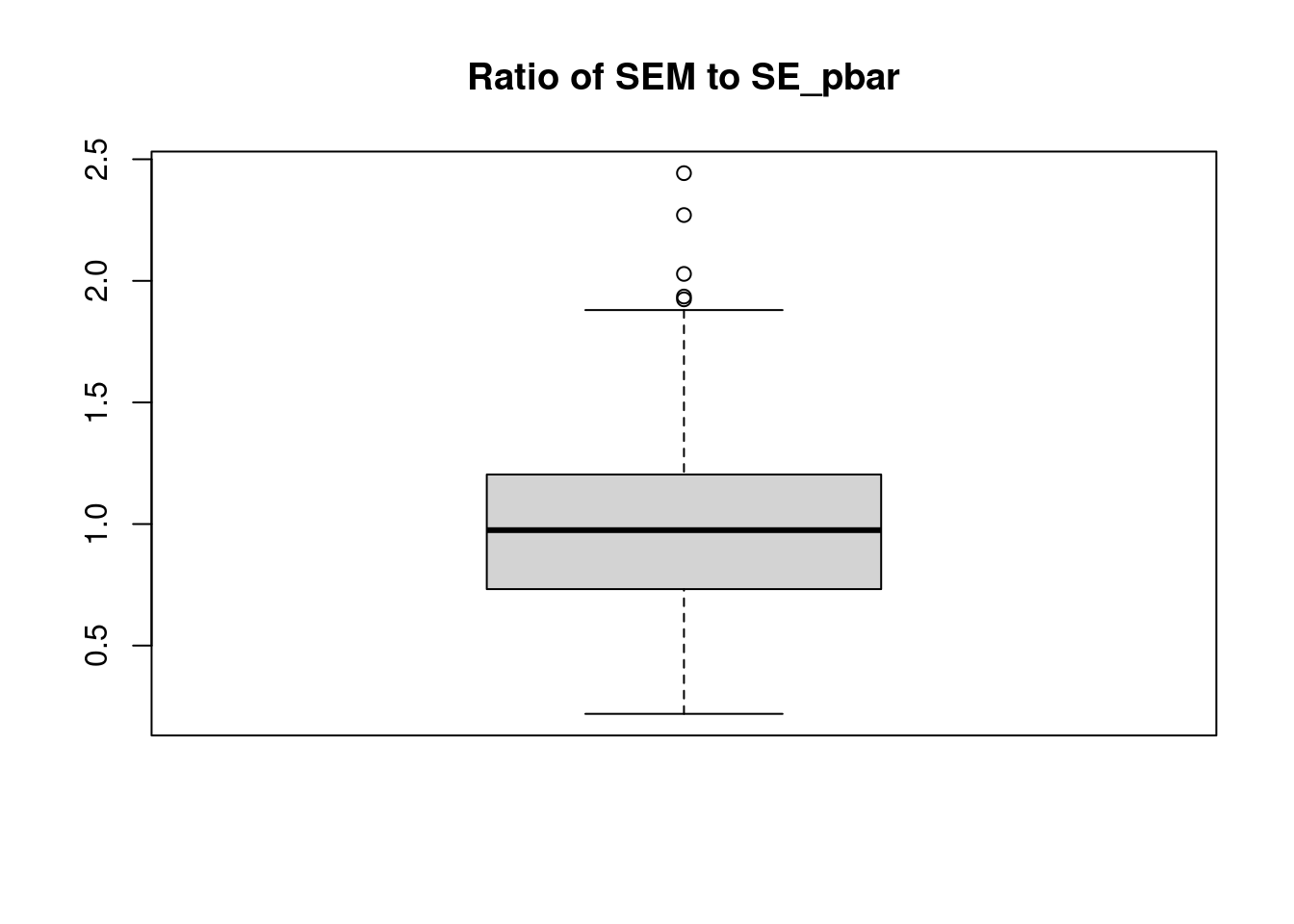
boxplot(res$SEM / res$SE_pbar, main = "Ratio of SEM to SE_pbar")